
Simulating colour blindness using MATLAB
4 August 2026
The term colour blindness encompasses a series of specific conditions in which an observer shows a reduced ability to discriminate between certain colours, compared with normal colour vision. The latter is characterised by the presence in the retina of three distinct types of cones (photosensitive cells), or trichromacy: S cones, which respond preferentially (though not exclusively) to short wavelengths of visible light (perceived as blue); M cones, which respond preferentially (though not exclusively) to medium wavelengths of visible light (perceived as green); and L cones, which respond preferentially (though not exclusively) to long wavelengths of visible light (perceived as red). In colour blindness (excluding achromatopsia, in which the entire retina lacks cones), the functioning of one of these cone types is altered, either due to anomalies (the most common case) or because it is absent from the retina altogether – dichromacies, among which we can distinguish protanopia (absence of L cones), deuteranopia (absence of M cones), and tritanopia (absence of S cones).
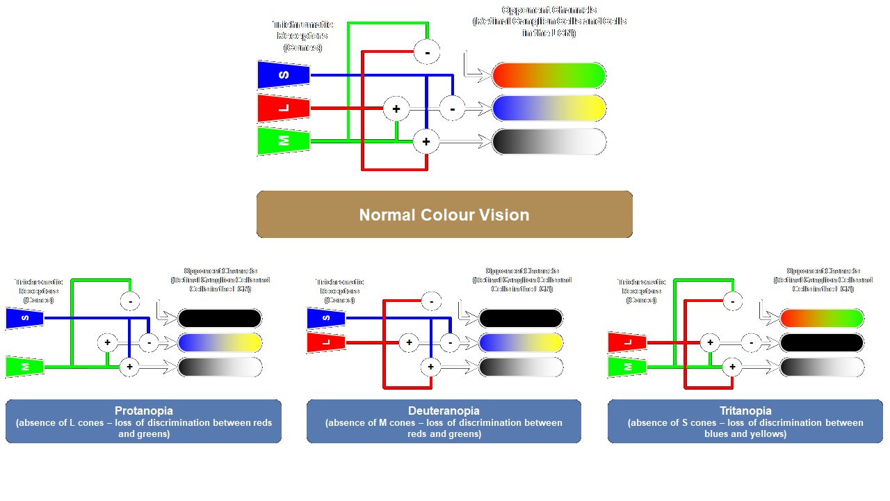
Based on this description, one might hypothesise that people with dichromacy would lose the ability to perceive the hues to which the missing cone is most responsive. That is, for example, a person with protanopia, lacking L cones in the retina, would show an inability to perceive red tones, to which those cones would respond preferentially. This is not, in fact, what happens. People with dichromacies show an inability to discriminate between two hues – that is, the perceptual losses occur in pairs: in protanopia and deuteranopia, the ability to discriminate between red and green tones is lost, and in tritanopia, the ability to discriminate between blue and yellow tones is lost. The reason for this stems from the fact that cone responses, although critical for colour perception, represent only the first step in a more complex sequence of information processing (see Figure 1). Thus, some ganglion cells, still within the retina, as well as neurons in the Lateral Geniculate Nucleus, carry out a reparameterisation of the responses of cone populations, resulting in what are called opponent channels. Some of these cells respond to the difference between the responses of L and M cones, effectively computing the relative amount of red or green. Others respond to the difference between the response of S cones and the combined response of L and M cones, resulting in the opposition between blue and yellow. Finally, others process the total amount of light, processing the responses of all cone types. In dichromacies, that is, in the absence of one of the three cone types, these opponent channels become compromised: in protanopia and deuteranopia, the absence of L or M cones, respectively, makes it impossible to process the opposition between red (L cones) and green (M cones); in tritanopia, the absence of S cones similarly makes it impossible to process the opposition between blue (S cones) and yellow (M + L cones).
Note that the description "inability to discriminate between red and green hues" applies to both protanopia and deuteranopia, suggesting that the two conditions produce exactly the same perceptual effect. This is not entirely true – although this description applies qualitatively to both conditions, there are subtle quantitative differences. With this caveat in mind, the exercise that follows will simulate dichromacies only qualitatively, and as a first approximation, without attempting to model the distinctions between protanopia and deuteranopia. Although it is perfectly possible to simulate dichromacies with a greater degree of precision (and there are several tools online that do so), this would involve an increased degree of complexity, and a consequent compromise to the pedagogical value expected of an introductory course in the psychology of perception, for which this exercise is intended. Despite this caveat, the procedures that follow may be useful in contexts where the distinction between protanopia and deuteranopia is not critical, such as, for example, testing colour schemes to ensure their suitability for people with colour blindness. To carry out this exercise, it is first necessary to install the 'Image Processing Toolbox' Add-On in MATLAB. Additionally, any digital photograph intended for use in the colour-blindness simulation should be copied to MATLAB's active folder.
The underlying logic used here is as follows: the colours of an image, encoded in the RGB system, will be converted to the CIELAB (or L*a*b*) system, which represents colours across three opponent channels: (i) Luminance (L*), (ii) red-green (a*), and (iii) blue-yellow (b*). These three channels are encoded, in MATLAB, in the third dimension of a matrix, similarly to what happens in the RGB system. Once this conversion has been made, the second (a*; red-green, simulating the result of protanopia and deuteranopia) or third (b*; blue-yellow, simulating the result of tritanopia) layer of this third dimension will be selectively eliminated (by changing its values to 0). The result will then be converted back to RGB for visual display.
Thus, we begin by importing a digital image as an H × V × 3 matrix, where H and V specify the horizontal and vertical dimensions of the photograph, with the third dimension encoding the intensity of the red, green, and blue (RGB) channels. This matrix is then normalised (the values of the R, G, and B channels are converted from bytes, between 0 and 255, to values between 0 and 1) and converted to the CIELAB system.
Photo = imread('name.extension');   % Import image as a matrix - Replace "name" and "extension" by the corresponding values of the image file
Norm = im2double(Photo);            % Normalise the matrix values (0-1)
LAB = rgb2lab(Norm);                % Convert the image, from RGB, to CIELAB
Next, two copies of the LAB matrix are created, one in which the b* (blue-yellow) values are changed to 0 – LAx – and another in which the a* (red-green) values are changed to 0 – LxB.
LAx = LAB;                          % Duplicate the LAB matrix under the name LAx
LAx(:,:,3) = 0;                     % Change the values of the third layer of the third dimension (b*; blue-yellow) to 0

LxB = LAB;                          % Duplicate the LAB matrix under the name LxB
LxB(:,:,2) = 0;                     % Change the values of the second layer of the third dimension (a*; red-green) to 0
The LxB and LAx matrices are then converted to RGB, for visual display.
ProtDeut = lab2rgb(LxB);            % Convert the LxB matrix to RGB under the name ProtDeut
Trit = lab2rgb(LAx);                % Convert the LAx matrix to RGB under the name Trit
To view the results, alongside the original image, use the following commands:
figure;
subplot(1,3,1)
image(Photo)
subtitle('Normal Vision')
subplot(1,3,2)
image(ProtDeut)
subtitle('Protanopia and Deuteranopia')
subplot(1,3,3)
image(Trit)
subtitle('Tritanopia')
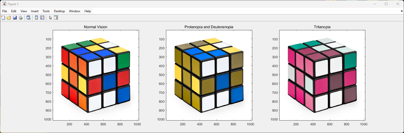
The result should be similar to that in Figure 2.
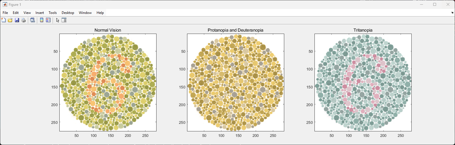
An interesting exercise, which may help clarify some aspects of colour vision, consists of repeating this exercise using patterns from the Ishihara test, used for diagnosing colour blindness, as the initial image (see Figure 3).