
The Marr & Poggio Cooperative Algorithm – Flatland version
18 September 2026
You, who are blessed with shade as well as light, you, who are gifted with two eyes, endowed with a knowledge of perspective, and charmed with the enjoyment of various colours, you, who can actually SEE an angle, and contemplate the complete circumference of a Circle in the happy region of the Three Dimensions – how shall I make it clear to you the extreme difficulty which we in Flatland experience in recognizing one another's configuration? (Abbott, 1884)
The cooperative algorithm for solving binocular disparities, proposed by David Marr and Tomaso Poggio in 1976, constitutes an unavoidable landmark in research on binocular perception. It shows, for the first time, how the so-called Correspondence Problem – which elements of the optical image in one eye correspond to which elements of the optical image in the other eye, an inverse and underdetermined problem – can be solved in computational terms.
Although the solution proposed by Marr and Poggio is not the only one in the relevant literature and, moreover, may not be at all the one actually implemented by the visual system (for a general, albeit no longer recent, review, see Bruce, Green, & Georgeson, 2003), it represents a singular pedagogical opportunity to show how the classical notion of unconscious inference, proposed by von Helmholtz at the end of the nineteenth century, can be instantiated in a computationally and neurophysiologically plausible algorithm (cf. Palmer, 1999). In this sense, within a course on perception, the cooperative algorithm can constitute an important turning point between classical conceptions and modern approaches to the study of perception, revealing the conceptual continuities between theories that are chronologically distant. Moreover, given its simplicity, an accessible version can readily be programmed with only a few lines of MATLAB code, fostering active teaching and learning methodologies, as will be shown below.
Given its essentially pedagogical purpose, we shall consider here not beings moving in a three-dimensional world, like us (a MATLAB function implementing the cooperative algorithm for solving three-dimensional random-dot stereograms can be found here), but rather inhabitants of the hypothetical Flatland (Abbott, 1884). This simplification, useful for teaching and understanding the algorithm, does not compromise the core idea, since expanding the algorithm from a two-dimensional world to a three-dimensional world is almost merely a matter of scale. Before guiding the reader through the implementation of the algorithm in MATLAB, it is important to provide some preliminary explanations – an informed reader may simply skim through these and proceed to the following section; conversely, a reader who merely wishes to understand the basic logic of the cooperative algorithm can focus on the following section and ignore the one that follows. Obviously, it is hoped that an interested reader will benefit from reading both sections carefully.
The Correspondence Problem and the Cooperative Algorithm
To make concrete the basic problem that the algorithm seeks to solve, consider perhaps the most famous inhabitant of Flatland, the estimable lawyer, the square A. Square. In Figure 1 we see, at the bottom, the frontal part of A. Square, repeated in all three panels. Within it, we can see the retinas of both his "eyes", fixated on the point marked with a cross higher up in the figure and, therefore, immediately in front of A. Square (obviously, we shall disregard here any biological and/or biomechanical considerations concerning the visual system of the inhabitants of Flatland; Abbott, in his fictional text, suggests that these beings possess only a single eye, a fact that we shall ignore for the sake of the topic at hand). By "eyes" (from now on we shall dispense with the quotation marks) we mean here two line segments, consisting of sequences of photoreceptor cells, represented in Figure 1 as rows of small squares. As in the three-dimensional world, these cells respond to light reaching them from particular visual directions, represented in the Figure by dashed arrows. When A. Square fixates any point in his world, light reflected by lines within his two-dimensional space (the equivalent of surfaces in our world) falls upon the photoreceptor cells within his eyes, generating an optical image in each of them. In Figure 1, we can see that his two eyes are registering two optical images – some retinal cells signal a golden point, others a blue point. However, and this is the important aspect, the two optical images are not exactly identical to one another – there are small differences corresponding to binocular disparities. For example, the fifth cell from the left registers a golden point in the left eye, whereas the corresponding cell in the right eye registers a blue point – this occurs when a distal object in A. Square's visual field is either closer to or farther from him than the fixation point. This means that the golden point in the fifth cell of the left eye is capturing the same light as one of the golden cells in the right eye, which may be further to the left (crossed disparity, if the distal point is closer to A. Square) or further to the right of that eye (uncrossed disparity, if the distal point is farther away from A. Square).
Determining which retinal point in the left/right eye corresponds to which retinal point in the right/left eye is what we call the Correspondence Problem. The reason why this is an underdetermined problem lies in the fact that any point in one eye may correspond to any other point in the other eye. In Figure 1, this means that the intersection between any two visual directions from the two eyes (intersections of the dashed arrows) may potentially be a genuine correspondence. This ambiguity multiplies when all points are considered – given any two optical images, one from each eye, there are countless possible solutions (which points in two-dimensional space are or are not occupied by an object), of which only one is veridical. Each of the three panels in Figure 1 shows, for the optical images represented, one of the countless possible solutions – note that the optical images, that is, what A. Square actually sees through each of his eyes, are always exactly the same in all three panels; however, what is actually in front of A. Square, in his two-dimensional world, may be a cloud of points at different depths, as in panel A, several line segments at different depths, as in panel B, or one line closer to him and two lateral lines slightly farther back, as in panel A. It is important to emphasise that these are only three possible solutions among countless possibilities, which is why the problem initially appears to be virtually insoluble.
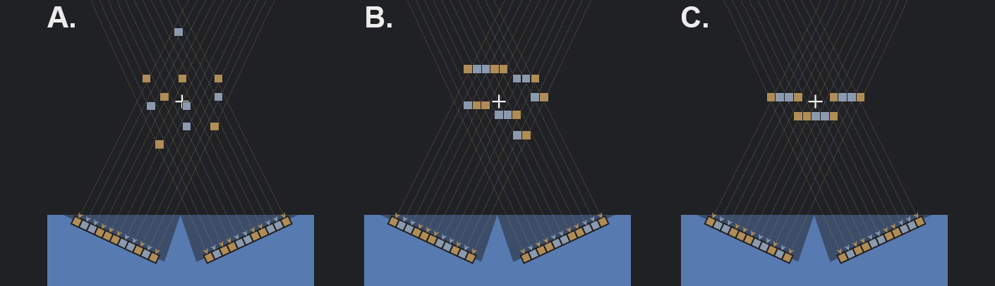
Solving the Correspondence Problem therefore requires imposing constraints within the universe of possible solutions, ideally until only one remains that, at least in most situations, represents the veridical configuration of distal points in the world. A first constraint has already been considered by us in Figure 1, albeit implicitly: a point in the world cannot appear to have one colour in one eye and another, different colour in the other – in other words, points resulting from the intersection of visual directions with different luminances can be excluded (in Figure 1, any intersection between golden arrows and blue arrows, and vice versa). This partially reduces the set of potential solutions, but does not solve the Correspondence Problem, since countless plausible solutions still remain. A second constraint, which we shall not consider here, consists in delimiting a region in space around the fixation point (or, strictly speaking, around the horopter) and considering only the solutions contained within it – the logic here is to exclude points that are excessively near to or far from the observer relative to the fixation point, through a stereoscopic fusion threshold, on the grounds that, if there is an object more or less distant than the current fixation point, the latter can be adjusted by fixating a new point in the world. This is indeed what happens, but the Correspondence Problem nevertheless remains, since countless potential solutions remain within this limit.
Marr and Poggio's fundamental intuition was that the very nature of the world we inhabit provides additional constraints, in the form of natural regularities – insofar as the visual system rests on certain plausible, but nevertheless inferential, assumptions about the solutions to be expected in the world, a considerable number of potential solutions can be eliminated, thereby solving the problem. This basic idea is essentially equivalent to von Helmholtz's notion of Unconscious Inference.
More specifically, in the cooperative algorithm, Marr and Poggio propose two constraints: (i) continuity assumption and (ii) uniqueness constraint or opacity assumption. The first – the continuity assumption – rests on the observation that, in our world (and, presumably, in Flatland), matter is cohesive and, therefore, objects in the world consist of continuous surfaces (or lines, in Flatland). Put differently, if a given point is a genuine correspondence, then adjacent points at a similar distance are also more likely to be genuine correspondences. This constraint is embodied in the algorithm by excitatory connections between equidistant and adjacent locations, as we shall see below. The second constraint – the opacity assumption – follows from the observation that, in our world (and, once again, in Flatland), matter tends to be opaque (with the exception of glass and translucent surfaces – I cannot conceive of an equivalent in Flatland, so we can ignore them entirely) and, therefore, along any visual direction only a single point can be a genuine correspondence (uniqueness). That is, in other words, if a point is a genuine correspondence, then correspondences immediately behind it, as seen by either eye, cannot be genuine (because they are occluded by it); similarly, correspondences immediately in front of it, along the same visual direction, cannot be genuine because, otherwise, we would see the latter rather than the former (which would be occluded). In Figure 1, the solution in panel B respects the continuity assumption, but violates the opacity assumption – the indicated correspondences form locally continuous line segments, but with some in front of others, which would only be a valid solution if they were entirely transparent (and therefore invisible). The solution in panel A, on the other hand, violates the continuity assumption, although not the opacity assumption – all points in the cloud occupy a unique position along each visual direction, but are isolated from one another, with no adjacent points. Finally, the solution in panel C respects both assumptions – this may be why it perhaps appeared to the reader as the most likely or plausible solution, and the reasons for this should now be clear.
Figure 2 schematises how these assumptions can be implemented in an algorithm. Panel A represents the space in which the necessary computations will be performed – this results from the intersection of the visual directions of the left eye (rows of the matrix) and the right eye (columns of the matrix) of A. Square. Each cell of this matrix corresponds to a given distal location in space. The main diagonal, marked by a continuous blue line, represents those points in the distal field that stimulate corresponding points on the retinas of both eyes (the first receptor of the left eye and the first receptor of the right eye, the second receptor of the left eye and the second receptor of the right eye, and so forth). This line is called the horopter and comprises all points that are at the same distance from the observer as the fixation point. Consequently, points closer to the bottom-left and top-right corners of the matrix than the horopter represent, respectively, locations closer to the observer (resulting in crossed disparities) and locations farther from the observer (resulting in uncrossed disparities), as indicated by the blue dashed bidirectional arrow. This matrix can be thought of as representing a population of neurons in A. Square's brain – the activation of any one of these neurons represents the perception of a distal point at the corresponding depth.
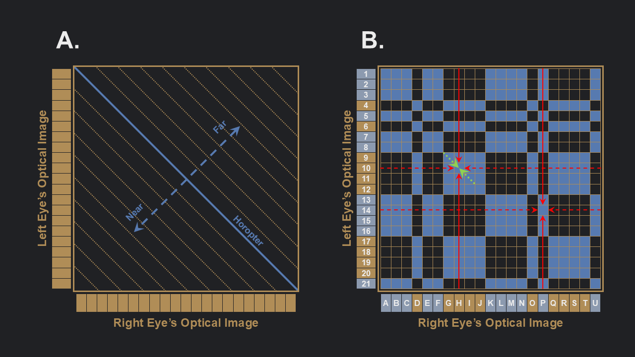
Panel B of Figure 2, in turn, shows the same matrix, but now with some active neuronal cells (represented in blue). The active neurons are those that have the same luminance in both eyes, which provides a first approximation to a solution. Consider cell H10 (column H and row 10). In the same column (H), that is, along the same visual direction as photoreceptor H of the right eye, there are another 9 cells that are also active. Similarly, in the same row (the visual direction of photoreceptor 10 of the left eye), there are 9 other active cells. In total, therefore, we have 18 cells sharing the same visual direction as cell H10 – in accordance with the opacity assumption, the latter will be "punished" by the others (e.g., through inhibitory connections) for being active (of course, it also contributes to the "punishment" applied to the others), causing its activation to decrease proportionally to the number of inhibitory connections. On the other hand, cell H10 has active cells at adjacent locations and at the same distance (G9 and I11) – under the continuity assumption, these cells will reinforce cell H10 (excitatory connections), causing its activation to increase. Now consider cell P14 – by the same reasoning, 18 cells along the same visual directions will decrease its activation (opacity assumption); however, unlike cell H10, it has no adjacent cell at the same distance that promotes its activation. This means that both cell H10 and cell P14 will experience the same magnitude of inhibition, but only the former will have some excitatory connections that partially compensate for the inhibition. The balance between excitatory and inhibitory connections, depending on the weight assigned to each of them, will determine whether the cell becomes inactive or, conversely, remains active: cell P14 will probably become inactive; cell H10 will probably remain active.
The algorithm performs these computations not merely on a pair of cells, but on all of them. Additionally, the algorithm is iterative – that is, the same computations are successively performed on the result of the previous iteration until a stable solution is reached.
Flatland Version of the Cooperative Algorithm – MATLAB code
To implement the cooperative algorithm, we shall create a script that can be run with different optical images for both eyes (the input data on which the algorithm operates). To do so, begin by creating a new script in MATLAB from the Editor menu. All the code portions that follow should simply be copied into this script, maintaining their order.
A primeira parte do script, abaixo, irá definir alguns parâmetros básicos, como o sejam o peso e extensão (quão distantes podem estar células que inibam/excitem cada célula) das ligações excitatórias e inibitórias, o número de iterações, e alguns parâmetros para a função logística que determina a activação das células em cada iteração.
The first part of the script below defines some basic parameters, such as the weight and extent (i.e. the maximum distance between cells that inhibit or excite a given cell) of the excitatory and inhibitory connections, the number of iterations, and the parameters of the logistic function that determines the activation of each depth-encoding cell at each iteration. All these parameters can be changed, which may cause the algorithm to converge more or less rapidly to a solution (or fail entirely). The default values were determined by me through trial and error and seem to work reasonably well, but they could certainly be fine-tuned (indeed, the reader will later be invited to alter them in order to explore the efficiency of the algorithm). The first line merely determines the size of the retinas of both eyes based on the optical image provided for the left eye (which should be the same as that of the right eye; these optical images will be generated later). Finally, the last line initialises the depth matrix (similar to the one shown in Figure 2) to which the algorithm will be applied. This matrix initially consists entirely of 0s, indicating that all cells are inactive.
%% Part 1 - Define Parameters

retinaSize = size(LeftEye,2); % Determine the size of the retinas

excExtent = 21; % Extent of excitatory connections - must be an odd value
excWeight = 1; % Weight of excitatory connections

inhExtent = 101; % Extent of inhibitory connections - must be an odd value
inhWeight = 0.1; % Weight of inhibitory connections

threshold = 0.5; % Central parameter of the logistic function governing the degree of activation of the cells at each iteration
slope = 0.05; % Slope parameter of the logistic function governing the degree of activation of the cells at each iteration

nIterations = 5; % Number of iterations

DepthMap = zeros(retinaSize); % Initialise the depth matrix
Next, the cells in this matrix that, based solely on the luminance registered by the photoreceptors of the retinas, represent possible correspondences are determined (that is, which cells have the same value in both retinas).
%% Part 2 - Activate cells with equal luminances in both eyes

% For each cell in the depth matrix, activate (1) those that have
% the same luminance value in both eyes
for leftIndex = 1:retinaSize
 for rightIndex = 1:retinaSize
  if LeftEye(leftIndex) == RightEye(rightIndex)
   DepthMap(leftIndex,rightIndex) = 1;
  end
 end
end
The following section effectively implements the cooperative algorithm and is therefore relatively long. Essentially, the lines of code below begin by generating two filters, one inhibitory and the other excitatory, which will be used to perform iterative convolutions of the depth matrix (effectively calculating, for each cell, the magnitude of inhibition and excitation). These filters embody the assumptions of continuity and opacity. Given the structure of the depth matrix, the inhibitory filter is simply a cross (+) of 1s (the remaining cells are 0s) – with the convolution, all cells in the same column and row as the target cell (excluding the target cell itself, to prevent self-inhibition, and those farther away than the extent defined above) will be multiplied by 1; the sum of the resulting values represents the total inhibitory connections of the target cell (i.e. the cell will be inhibited in proportion to the total activation of other cells in the same row and column). Similarly, the excitatory filter consists of a main diagonal of 1s (the remaining cells are 0s) – with the convolution, all cells on the same main diagonal as the target cell (excluding the latter, to prevent self-excitation, and those farther away than the extent defined above) will be multiplied by 1; the sum of the resulting values represents the total excitatory connections of the target cell (i.e. the cell will be activated in proportion to the total activation of other cells on the same main diagonal). Following the convolutions, two new matrices will be obtained: one representing the magnitude of excitation for each cell in the depth map, and the other representing the magnitude of inhibition. These two matrices will be weighted using the weights defined above to adjust the degree of activation of each depth cell and subjected to a logistic function that amplifies the degree of inhibition/excitation, in order to facilitate convergence towards a solution and based on the previously defined parameters. The same process is then repeated on the resulting output, as many times as specified by the number of iterations.
For teaching purposes, the following lines also include some instructions for generating an image that will be updated at each iteration (with a half-second interval imposed), appropriately identified as such by a comment. In this way, one can see the evolution of the depth matrix, with some cells disappearing and others becoming active, until the final solution is reached. The lines of code relating to visualisation can, if desired, be removed (in which case the code runs only the algorithm).
Finally, a small note. For the excitatory filter, the MATLAB function eye is used – it simply returns an identity matrix of the specified size (that is, a matrix with 1s on the main diagonal; in matrix algebra, the identity matrix is the neutral element of multiplication). In the present context, eye should not be confused with anything relating to the virtual eyes being considered here.
%% Part 3 - Cooperative Algorithm

% Excitatory filter - Continuity Assumption
ExcFilter = eye(excExtent); % Reward correspondences on the same negative diagonal (equidistant)
ExcFilter((excExtent+1)/2,(excExtent+1)/2) = 0; % Prevent self-excitation

% Inhibitory filter - Opacity/Uniqueness Assumption
InhFilter = zeros(inhExtent); % Initialise the filter
InhFilter(:,round(inhExtent/2)) = ones(1,inhExtent); % Penalise correspondences on the same row (same visual direction in the left eye)
InhFilter(round(inhExtent/2),:) = ones(inhExtent,1); % Penalise correspondences on the same column (same visual direction in the right eye)
InhFilter(round(inhExtent/2),round(inhExtent/2)) = 0; % Prevent self-inhibition

State = zeros(retinaSize,retinaSize,nIterations+1); % Initialise a 3D matrix that will record the state of the depth matrix at each iteration
State(:,:,1) = DepthMap; % Store initial state (based on equiluminance)

% Cooperative Algorithm

for i = 1:nIterations
 colormap gray % For visualisation only - remove if unnecessary
 imagesc(State(:,:,i)) % For visualisation only - remove if unnecessary
 axis equal % For visualisation only - remove if unnecessary
 pbaspect([1 1 1]) % For visualisation only - remove if unnecessary
 pause(0.5); % For visualisation only - remove if unnecessary

 ExcMap = conv2(DepthMap, ExcFilter, "same"); % Calculate the magnitude of excitation for each cell
 InhMap = conv2(DepthMap, InhFilter, "same"); % Calculate the magnitude of inhibition for each cell
 DepthMap = DepthMap + excWeight * ExcMap - inhWeight * InhMap; % Calculate activation by weighting excitation and inhibition
 DepthMap = max(DepthMap, 0); % Eliminate any negative values (no cell can have negative activation)
 DepthMap = DepthMap ./ max(1e-6, max(DepthMap(:))); % Normalise the values to a scale from 0 to 1
 DepthMap = 1 ./ (1+exp(-((DepthMap-threshold)/slope))); % Logistic function to accelerate convergence
 State(:,:,i+1) = DepthMap; % Store the result of this iteration
end
The following code section is entirely optional. It merely generates a figure showing, in separate panels, the initial solution (determined by equiluminances), the solution after approximately 1/3 of the number of iterations, approximately 1/2 of the number of iterations, and the final solution (after the specified number of iterations has been completed).
%% Part 4 - Summary of the Evolution Across Iterations

figure
colormap gray
subplot(2,2,1)
imagesc(State(:,:,1))
axis equal
pbaspect([1 1 1])
title('Initial disparity map, based on luminance correspondences')
xlabel('Right Eye Optical Image')
ylabel('Left Eye Optical Image')
subplot(2,2,2)
imagesc(State(:,:,round((1/3) * nIterations)+1))
axis equal
pbaspect([1 1 1])
title(['State after ', num2str(round(((1/3) * nIterations))), ' iterations'])
xlabel('Right Eye Optical Image')
ylabel('Left Eye Optical Image')
subplot(2,2,3)
imagesc(State(:,:,round((1/2) * nIterations)+1))
axis equal
pbaspect([1 1 1])
title(['State after ', num2str(round(((1/2) * nIterations))), ' iterations'])
xlabel('Right Eye Optical Image')
ylabel('Left Eye Optical Image')
subplot(2,2,4)
imagesc(State(:,:,nIterations+1))
axis equal
pbaspect([1 1 1])
title(['Final solution (', num2str(nIterations), ' iterations)'])
xlabel('Right Eye Optical Image')
ylabel('Left Eye Optical Image')
The script can now be saved in the active folder under whatever name is desired. The only thing remaining in order to see the cooperative algorithm in action is to have two matrices, each consisting of a single row of arbitrary length, representing the optical images of the left eye (designated LeftEye) and right eye (designated RightEye) of A. Square. For now, the reader can simply use the following example, entering the two lines below in the MATLAB command window (or, alternatively, in the first lines of the script, immediately before "Part 1") and then running the script (hiting the Run button in the Editor menu, making sure that the corresponding file is open and selected). These two matrices, consisting of 0s and 1s, represent the Flatland equivalent of a random-dot stereogram, in which 0 refers to a black dot and 1 to a white dot. In this particular case, the disparities introduced into the stereogram should result in the perception of a line segment, approximately in the middle of the visual field, closer to the observer and in front of a partially occluded line on the horopter (similar to panel C of Figure 1).
LeftEye = [1 1 1 0 0 1 1 0 1 0 1 0 1 0 0 0 1 0 0 1 1 0 0 1 1 0 1 0 0 0 0 0 0 0 0 1 1 0 0 1 0 0 1 0 1 0 0 1 1 0 1 1 0 1 1 1 0 0 0 0 1 0 0 0 1 0 1 0 0 0 1 0 0 1 1 0 1 1 0 0 1 1 0 0 1 1 1 0 1 1 1 0 0 0 1 1 0 1 1 1];

RightEye = [1 1 1 0 0 1 1 0 1 0 1 0 1 0 0 0 1 0 0 1 0 0 1 0 1 0 0 1 1 0 1 1 0 1 1 1 0 0 0 0 1 0 0 0 1 0 1 0 0 0 1 0 0 1 1 0 1 1 0 0 0 1 1 0 0 1 0 1 1 0 0 0 1 1 1 0 1 1 0 0 1 1 0 0 1 1 1 0 1 1 1 0 0 0 1 1 0 1 1 1];
If the reader wishes to generate other random-dot stereograms, the following code can be used, saved in a separate script. This generates two optical images, one for each eye, encoding binocular disparities in a line segment defined by several parameters: LineDisparity specifies the magnitude and direction of the binocular disparity (negative/positive values make the line appear nearer/farther away, respectively, and the greater the absolute value, the greater the apparent depth); LineStart defines the horizontal location of the line segment, further to the left or right relative to the observer; finally, LineLength specifies the extent of the line segment subject to binocular disparity.
RetinaSize = 100;

LineLength = 40;
LineStart = 40;
LineDisparity = -20; % Negative values = closer; positive values = farther away

RightEye(LineStart+LineDisparity:LineStart+LineLength+LineDisparity-1) = LeftEye(LineStart:LineStart+LineLength-1);

if LineDisparity < 0
    RightEye(LineStart+LineLength+LineDisparity\:LineStart+LineLength-1) = randi([0 3],1,-LineDisparity);
end

if LineDisparity > 0
    RightEye(LineStart\:LineStart+LineDisparity-1) = randi([0 3],1,LineDisparity);
end
The reader is invited to generate several stereograms and test them with the iterative algorithm, changing its parameters. Here are some questions that can be explored in this way:
- What happens when inhibition or excitation is given too much weight?
- How effective/ineffective is the algorithm when the extent of inhibitory or excitatory connections is decreased/increased?
- How does the weight of inhibition and/or excitation interact with the extent of inhibitory and excitatory connections?
- How long must the line segment subject to disparity be for it to be correctly detected by the algorithm?
- Under what conditions more or less iterations are required?
- How much better or worse does the algorithm perform when the parameters of the logistic function that determines the degree of activation of the cells at each iteration are changed?
Some Final Notes
As stated at the very beginning, this implementation of the Cooperative Algorithm is intended entirely for pedagogical purposes and therefore incorporates several simplifications. The first of these, although innocuous, is naturally the fact that it is applied to inhabitants of Flatland. Another, related to the way in which the assumption of continuity is implemented, nevertheless deserves a few lines. In the present case, only points that are exactly equidistant benefit from mutual excitation, which means that only lines orthogonal to the cyclopean line of sight are perceived. Points belonging to a line with a slight inclination are subject only to inhibition, resulting in an inaccurate solution. A more careful implementation of the algorithm would require a greater density of excitatory connections to be considered, not only between points at exactly the same distance but also between points at slightly greater or smaller distances. The same applies, incidentally, to the three-dimensional version of the algorithm: not all surfaces are parallel to the fronto-parallel plane, and they may perfectly well be viewed at some angle, which should be taken into account. This caveat, relevant from a computational standpoint, amounts to no more than this brief note from a pedagogical perspective.
Bibliography
-
Abbott, E. A. (1884). Flatland: A Romance of Many Dimensions. Feedbooks.
-
Bruce, V., Green, P. R., & Georgeson, M. A. (2003). Visual Perception: Physiology, Psychology and Ecology (4th ed.). Psychology Press.
-
Marr, D., & Poggio, T. (1976). Cooperative Computation of Stereo Disparity. Science, 194(4262), 283–287.
-
Palmer, S. E. (1999). Vision Science: Photons to Phenomenology. The MIT Press.